The article is my own understanding, any comment to this article is welcomed, and please feel free to approach me if you have any question.

In the era of big data, gigabytes or terabytes of data are available day by day. Given a model, it raises our concerns that we need to make sure the parameters are estimated correctly to monitor or predict the performace. Take financial industry as an instance, according to the Basel Accord, banks are required to calibrate the model parameters periodically in preparing the capital requirements for the sake of the accuracy and time-dependence of the model.

The difficulties in estimation are obvious. Sequential data arrive every day, and we need to assure the effectiveness of the parameters for a concrete model. However, if there is a large batch of data, it is quite time-consuming to figure out the correct parameters. Hence, Sequential Monte Carlo(hereinafter SMC) is introduced in such cases. SMC is an useful estimation technique for dynamic systems.

To introduce SMC, we must have basic understanding about bayesian statistics. Firstly, let us talk about prior distribution, it is our belief about an uncertain quantity before some evidence is taken into account. For example, you are going to toss a coin, the basic belief is that there are two outcomes(head, tail) and the probability of each outcome is the same. Secondly, a likelihood function. It is defined as a function about a parameters given some specified data or other evidence. To simplied the form of the likelihood function, sometimes we will take a logarithm to the likelihood functiom. Finally, posterior distribution, the target distribution we want to optimize, is the distribution of unknown quantities, regarded as random variables, given the observed evidence.

Then it comes to an equation below \[posterior \propto prior \times likelihood \]

To conclude, prior is what you know about parameters. Likelihood is how likely the data are if the parameters are given based on modeling assumption. Posterior, is the product of the prior and likelihood, representing the probability of parameters after taking obsevations into account.

Let me give some definition about the terms will be used in SMC. Let \(\pi(\theta)\) denote the prior. And Denote \(\mathcal{L}(X|\theta)\) the likelihood function and \(\gamma(\theta,X)\) is the posterior.Thus, we can devire \[\gamma(\theta,X) \propto \pi(\theta) \times \mathcal{L}(X|\theta)\]

Since the data come into system sequentially, we can change the notations a little bit. Now, \(\mathcal{L}_{n}(X|\theta)\) would be the likelihood given data coming during time \(n-1\) and time \(n\) and \(\gamma_n(\theta,X)\) would be the posterior distribution up to the time \(n\). After incorporating the time, the equation will be \[\gamma_n(\theta,X) \propto \pi(\theta) \times \prod_{t=1}^n\mathcal{L}_n(X|\theta)\]

To obtain the correct parameters, we can randomly generate \(K\) paritcles. Each partical contains a set of parameters. And there is a weight for each particle. A larger weight of a particle represents that the parameters in the particle can generate a high posterior. At initial, the role of the prior \(\pi(\theta)\) is to provide the initial particles which the algorithm can start and every particle has the same weight as the beginning. Then the particles can be showed as below. \[\theta^{(k,0)} \thicksim \pi(\theta), \omega^{(k,0)} = \frac{1}{K}\]

Once the initial partcles are determined. We can proceed to derive the parameters using Recursions. Let start at a random time \(n\). Suppose there are known particles and its corresponding weights \((\theta^{(k,n)} , \omega^{(k,n)}) \). During the time \(n\) and \(n+1\), there was a batch of data coming in and our purpose is to move from posterior distribution \(\gamma_n(\theta)\) to current posterior distribution \(\gamma_{n+1}(\theta)\). Sometimes, it is too ambitious to move directly from \(\gamma_n(\theta)\) to \(\gamma_{n+1}(\theta)\) as the two distributions are too fat from each other. Hence, a tempered bridge is built between the two densities and the particles are evolved through the resulting sequence of density.\[\overline{\gamma}_{n+1,p}(\theta) \propto \gamma_n(\theta) \times \mathcal{L}^{\xi_p}_{n+1}(\theta)\] \[for\ p = 0,...,P_{n+1}\]

Here, a bridge is built. When \(\xi_0=0\)

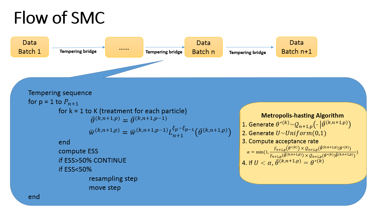
\[\overline{\gamma}_{n+1,0}(\theta)=\gamma_n(\theta)\]

when \(\xi_{P_{n+1}} = 1\) \[\overline{\gamma}_{n+1,P_{n+1}}(\theta)=\gamma_{n+1}(\theta)\] Here, \(P_{n+1}\) is the length of tempered bridge. For \(p\) between 0 and \(P_{n+1}\) , \(\xi_p\) is a sequence from 0 to 1. Through the built tempered bridge, we can proceed to reach \(\gamma_{n+1}(\theta)\) using a reweighting and resampling step.

Since the introduction of tempered bridge, we would like to incorporate \(p\) into particles and obtain an updated particle \(\overline{\theta}^{(k,n+1,p)}\) meaning the the parameters in the particle \(k\) at the sequence \(p\) up to time \(n+1\). Given the definition, we can proceed to the \(Reweighting Step\). In the \(Reweighting Step\), each particle at sequence \(p\) will follow the praticle at sequence \(p-1\) and its corresponding weight will change using an importance sampling principle.

\[\overline{\theta}^{(k,n+1,p)} \ = \ \overline{\theta}^{(k,n+1,p-1)}\]

\[\overline{\omega}^{(k,n+1,p)}\ = \ \overline{\omega}^{(k,n+1,p-1)} \times \frac{\overline{\gamma}_{(n+1,p)}(\overline{\theta}^{(k,n+1,p)})}{\overline{\gamma}_{(n+1,p-1)}(\overline{\theta}^{(k,n+1,p)})} = \overline{\omega}^{(k,n+1,p-1)} \times \mathcal{L}^{\xi_{p+1} - \xi_{p}}_{n+1}(\overline{\theta}^{(k,n+1,p)})\]

Since the effect of importance sampling, a higher weight will be assigned to a particle which can better fit the likelihood, meanwhile, a poor particle's weight becomes smaller. After several steps of tempered bridge, most particle's weights will be concentrated on a small number of particles, meaning there is a poor diversification. To aviod particle impoverishment in sequential importance sampling, Effective Sample Size is introduced. \[ESS = \frac{(\sum_{k=1}^{K}\overline{\omega}^{(k,n+1,p)})^2}{\sum_{k=1}^K(\overline{\omega}^{(k,n+1,p)})^2}\] It measuares the concentration of the particles taking weights into account. If the ESS calculated is smaller than a predetermined value, meaning the particles are impoverishment. Hence, a \(Resampling Step\) and move step are required to solve such problems.

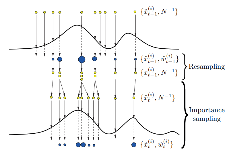
Since the weights of the particles are totally different and are concentrate on either high or low weights after several tempered steps. Resampling Step can help to generate particles with uniform weights. We adopt weight sampling and the particles are resampled proportional to their weights. \[\overline{\theta}^{(k,n+1,p)} = \overline{\theta}^{(I^{(k,n+1,p)},n+1,p)}\]

\[\overline{\omega}^{(k,n+1,p)} = \frac{1}{K}\]

After the resampling step, we obtain a new set of particles. However, all the particles are sampled from the previous one. So we need a move step to enrich the support of the particle cloud to find the potential better results. Typically, a Metropolis-Hastings algorithm is used. The Metropolis-Hastings algorithm is a Markov Chain Monte Carlo method for obtaining a sequence of random sample from a probability distribution for which direct sampling is difficult. The general procedures are listed below.

1. Generate samples from the proposal distribution, propose \(\theta^{*(k)} \thicksim \mathcal{Q}_{n+1,p}(\centerdot|\overline{\theta}^{(k,n+1,p)})\)
2. Generate a random variable \(U \thicksim uniform(0,1)\)
3. Compute the acceptance rate \[\alpha = min(1,\frac{\overline{\gamma}_{(n+1,p)}(\theta^{*(k)}) \times \mathcal{Q}_{n+1,p}(\overline{\theta}^{(k,n+1,p)}| \theta^{*(k)} ) }{\overline{\gamma}_{(n+1,p)}(\theta^{(k,n+1,p)}) \times \mathcal{Q}_{n+1,p}(\theta^{*(k)} | \theta^{(k,n+1,p)} ) })\]
4. If \(U<\alpha\), \(\overline{\theta}^{(k,n+1,p)} = \theta^{*(k)} \)

The figure above gives us a very comprehensive illustration about the the procedure Resampling and Move Step work.

Let summarize the procedures of a typical SMC.Please see the general pseudo code below.

Talking about the SMC is rather unintuitive. So I would like to use a simple case to demonstrate it.

A linear model estimation will be performed under SMC. Suppose the linear model is \(y = \beta_0 + \beta_1 x\). In this case, since we do not have any idea about the parameters. We can simply assume that the parameters \(beta_0, beta_1\) follow a identical independent normal distribution. And the prior can be represented as \[\pi(\theta_i)\ \thicksim \mathcal{N}(0,\sigma_1^2)\ i.i.d. \ \ i=0,1\]

The likelihood function can be derived as \[lilelihood\ \propto \prod_{t = 1}^{n} exp(- \frac{(y_i\ -\ \beta_0 - \beta_1x_i)^2}{2\sigma_{2}^2})\]

Then the posterior is \[posterior \propto exp(-\frac{\beta_0^2+\beta_1^2}{2\sigma_1^2})\ \times\ \prod_{t=1}^{n}exp(- \frac{(y_i\ -\ \beta_0 - \beta_1x_i)^2}{2\sigma_{2}^2})\]

Let us further clarify other settings. We set the number of particles as \(K=1000\) and the length of tempered bridge as \(P_{n+1} = 1000\) so that the \(\xi_p\) is a sequence from 0 to 1 with an interval 0.001

Assuming the data arriving periodically, we can update the particles and their corresponding weights using a tempered bridge. The parameters in the particle and the weight will be listed following \[\overline{\theta}^{(k,n+1,p)} = \overline{\theta}^{(k,n+1,p-1)}\ k = 1,...,K\] \[\overline{\omega}^{(k,n+1,p)} = \overline{\omega}^{k,n+1,p-1}\ \times [\prod_{i=1}^{t_{n+1,N}}exp{-\frac{(y_i-\beta_0-\beta_1x_i)^2}{2\sigma_2^2}}]^{\xi_p-\xi_{p-1}}\] since the difference between \(\xi_p\) and \(\xi_{p-1}\) is a constant and the sum of weights for all particles equals to 1. The Effective Sample Size is calculated as \[ESS = \frac{1}{\sum_{k=1}^K(\overline{\omega}^{(k,n+1,p)})^2}\]

If the ESS for all particles is less than a predetermined value, we will resample the particles and adopt the Metropolis-Hastings algorithm.

To simplified, we propose a rbf kernel.\[\mathcal{K}(x,y) = exp(-\frac{||x-y||^2}{2\sigma^2_{kernel}})\] It is easier to get the acceptance rate \[\alpha = min(1,\frac{\overline{\gamma}_{n+1,p}(\overline{\theta}^{*(k)})}{\overline{\gamma}_{n+1,p}(\overline{\theta}^{(k,n+1,p)})})\]

Coding in Matlab:

test a random linear regression \(y = -1 +2\times x +\epsilon\)

x = randn(1000,1);

y = -1 + 2 * x

The results are

ans =

-0.9952 1.9922

Since SMC is a simulation-based technique. We can adpot some tricks to speed up the simulation process. Some possible methods are listed below.

1. The calculation of Posterior distribution takes most of the running time. If we migrate this process to GPU, it will greatly reduce running time.
2. There are some tradeoffs in SMC. Firstly, the negative relationship between running time and ESS. It means a smaller ESS will speed up the SMC. Secondly, a larger number of particles will slow down the SMC estimation but increase the accuracy of the estimation.
3. Choose the adequate prior and kernel function. For example, as for some constrained parameters, adpoting a log-normal as prior will be better than just normal one.
4. Using K-fold dupilcation

Reference:

1. National Unverisity of Singapore, Risk Management Insitute, RMI-CRI Technical Report[]
2. A introduction to Sequential Monte Carlo []